Experimenting with Shader Graph: Doing more with less


You can improve the runtime efficiency of your shader without sacrificing the quality of your graphics by packing physically based rendering (PBR) material information into a single texture map and layering it into a compact shader. Check out this experiment.
This experiment works in both the Universal Render Pipeline (URP) and High Definition Render Pipeline (HDRP). To get the most out of this article, you should have some familiarity with Shader Graph. If you are new to Shader Graph, please explore our resources for an introduction and more detail about this tool for authoring shaders visually.
When working with art assets in a terrain-like environment, multiple layers of tileable material are typically preferred as they produce better blending results. However, the GPU performance cost of multiple texture samples and growth of memory use with each layer added to the shader can be prohibitive for some devices and inefficient in general.
With this experiment, I aimed to:
- Do more with less
- Minimize the memory footprint and be frugal with texture sampling in representing a PBR material
- Minimize shader instructions
- Perform layer blending with minimum splat map/vertex color channels
- Extend the functionality of splat map/vertex color for extra bells and whistles
While the experiment achieved its goals, it comes with some caveats. You’ll have to set your priorities according to the demands of your own project in determining which trade-offs are acceptable to you.
Before layering, the first thing you need to do is figure out the PBR material packing. PBR material typically comes with the parameters for Albedo (BaseColor), Smoothness mask, Ambient Occlusion, Metalness, and Normal defined.
Usually, all five maps are represented in three texture maps. To minimize texture usage, I decided to sacrifice Metalness and Ambient Occlusion for this experiment.
The remaining maps – Albedo, Smoothness and Normal Definition – would traditionally be represented by at least two texture maps. To reduce it to a single map requires some preprocessing of each individual channel.
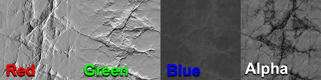
The final result of the PBR Material packed into a single texture. Red = dHdu (Derivatives Height Relative to the U direction) for Normal Definition#. Green = dHdv (Derivatives Height Relative to the V direction) for Normal Definition#. Blue = Linear Grayscale shade representing Albedo (color reconstructed in shader). Alpha = Linear Smoothness map (standard Smoothness map). Note: The texture is imported into Unity with sRGB unchecked and compressed with BC7 format. When porting to other platforms, switch to the platform-supported equivalent 4-channel texture format.
Processing the maps
Albedo
Albedo is normally defined as an RGB texture; however, many terrain-like materials (rock, sand, mud, grass, etc.) consist of a limited color palette. You can exploit this property by storing Albedo as a grayscale gradient and then color remapping it in the shader.
There is no set method for converting the RGB albedo to a grayscale gradient. For this experiment, The grayscale Albedo was created through selective masking of the original Albedo map channels and Ambient occlusion; to match the prominent color in the shader color reconstruction, just eyeball any manual adjustments.

Smoothness
Smoothness is considered very important for PBR material definition. To define smoothness more precisely, it has its own channel.
A simple multiplier was added to the smoothness in the shader for some variation in the material.

Normal definition
The Normal map is important for showing the detailed characteristics of a surface. A typical PBR Material uses a tangent space normal map. In this experiment, I chose a pre-converted derivatives map using surface gradient framework for the reasons below. (SeeMorten Mikkelsen’s surface gradient framework for more information).
To pre-convert tangent space normal maps to derivatives, use this Photoshop action.
Using a pre-converted Derivatives map has several advantages:
- Can be directly converted to surface gradient, using fewer instructions than a standard tangent space normal map, which requires derivatives conversion in the shader
- Can be stored in two channels (dHdu and dHdv), resulting in a lower memory and texture cache footprint in runtime
- Does not require blue channel reconstruction in the shader, which is typical when processing tangent space normal maps, since the surface gradient framework takes care of the normal reconstruction (fewer shader instructions)
- Works correctly when adjusted in Photoshop – that is, by blending, masking or reducing intensity – and does not require renormalization. For example, to reduce intensity, simply blend the map against RGB(128,128,0).
In conjunction with the surface gradient framework, the advantages further include:
- Normal bump information can be blended and composited in the shader the same way as albedo blend/composite, with the correct result.
- Increasing, reducing and reversing bump contributions is trivial and accurate.
But pre-converted derivatives from tangent space normal map also have some disadvantages:
- Using Photoshop conversion, normal definition gets clamped at an angle greater than 45 degrees, to balance precision in an 8-bit texture.
- Artists are used to working with tangent space normal maps and require the maps to be pre-converted via Photoshop as part of their workflow.
Note: Clamping at an angle greater than 45 degrees does not apply to shader-based derivatives conversion.
Depending on your use case, the limitation may have a lesser or greater effect. In this experiment, a normal direction less than 45 degrees does not have a noticeable negative impact on the end result. In fact, in this case it provides a benefit by reducing unwanted reflection from extreme normal direction.


The full unpacking process


For this experiment, I chose a tier-based layering method on a single channel remap. The Sub Graph does five linear interpolations (plus the base, forming six layers).
There are many ways to blend layer weights. This method has the simplicity of a single vector input, which suits the experiment goal. This allowed lots of layering without burning through multiple channels in splat maps or vertex channels.
The drawback of this method is that you cannot control the weight of an individual layer’s contribution. The blending will always be a transition from the previous layer. Depending on the use case, this can be a limiting factor compared to a traditional per-channel blend.

The Sub Graph to remap a single channel to represent the six layers.
The Sub Graph shown above is predefined for six layers of tier-based blending. To create more layers, divide 1 by the desired number of layers blended, subtract 1, and then remap each layer based on that value range.
For example, for a nine-layer blend material, each layer remap range is 1/(9-1) = 0.125.
Be aware that as you divide the single channel into smaller portions, you have less shading range.


Layer blending requires only a single channel (the red vertex channel). The remaining three vertex channels offer extra functionalities. The final Shader Graph produces results using the remaining vertex channels.
In this experiment, vertex painting was done inside Unity Editor using Polybrush (available from the Package Manager). Suggested Vertex Paint color palette for this shader.
Red: Used to weight the layer contribution. Red vertex channel painting demo
Green: Sets the surface gradient property, to flip, reduce or add normal bump contribution (remapped to -1 and 1).
- 0 reverses the normal bump (-1)
- 0.5 value zeroes out the normal bump (0)
- 1 sets the normal bump to the original value (+1).
Green vertex channel painting demo
Blue: Controls smoothness and surface gradient bump scale to create a wet water look
- 0 = no alteration
- 255 = maximum smoothness and flat normal map (wet look)
Blue vertex channel painting demo
Alpha: Controls the weight of the Albedo layer, setting the base color to white,with the contribution based on the y axis of the surface normal. It does not alter the smoothness and takes advantage of the original surface layer smoothness and bump property.
- 0 = no snow
- 255 = solid snow
Alpha vertex channel painting combined with previous channels to showcase how the whole layers interact with the snow
The combined results of the different vertex painting channels:
You can adjust the shader blending method and the settings for the various vertex channel/splat map functionalities according to your project’s requirements.
The purpose of this experiment was to extend the functionality of the Shader Graph while minimizing resources. The texture was preprocessed and unpacked, but is there a payoff in runtime efficiency?
Performance profiling shows the efficiencies these efforts produced.
A standard six-layer blend shader was created for comparison with the compact six-layer blend shader. Both shaders were created using an identical blending method with the same functionalities. The main difference is that the standard shader uses three different textures to represent a single layer.
For profiling, a single mesh was rendered on screen with blend material using the Universal Render Pipeline in the targeted platform.
Mobile memory and performance profile
Texture compression for mobile (Android):
Standard PBR with Albedo, Mask and Normal map at 1024x1024 for mobile:
- 6x Albedo map ASTC 10x10 = 6x 222.4 KB
- 6x Mask map ASTC 8x8 = 6x 341.4 KB
- 6x Normal map ASTC 8x8 = 6x 341.4 KB
Total Texture memory usage 5.431 MB
Compact PBR at 1024x1024 for mobile:
- 6x PackedPBR Texture ASTC 8x8 = 6x 341.4 KB
Total Texture memory usage 2.048 MB
With the compact six-layer material, there is approximately 62% Less texture memory consumption on Mobile (Android), savings of more than half. Mobile Android/Vulcan with Adreno 630 (Snapdragon 845); Snapdragon profile results:
- Approximately 70% less texture memory read in runtime.
- Standard took 9971020 clocks to render.
- Compact took 6951439 clocks to render.
Compact material renders on screen approximately 30% faster. Profiling result from Snapdragon Profiler.
PC memory and performance profile
Standard PBR with Albedo, Mask and Normal map at 1024x1024:
- 6x Albedo map DTX1 = 6x 0.7 MB
- 6x Mask map DXT5/BC7 = 6x 1.3 MB
- 6x Normal map DXT5/BC7 = 6x 1.3 MB Total Texture memory usage 19.8 MB
Compact PBR at 1024x1024:
- 6x PackedPBR Texture BC7 = 6x 1.3 MB
Total Texture memory usage 7.8 MB
The compact six-layer material uses 60% less texture memory consumption on PC (savings of more than half).
PC laptop with Radeon 460 Pro rendering at 2880x1800; RenderDoc profile results:
- Draw Opaques for standard 6-layer blend: 5.186 ms.
- Draw Opaques for compact 6-layer blend: 3.632 ms. Compact material renders on screen approximately 30%* faster. *RenderDoc profile value fluctuates; 30% is an average of samples.
PC desktop with nVidia GTX 1080 rendering at 2560x1440; nSight profile results:
- Render Opaques for standard 6-layer material: 0.87 ms
- Render Opaques for compact 6-layer material: 0.48 ms
Compact material renders on screen approximately 45% faster. Profiling results from nSight.
Console performance profile
On PlayStation 4, using compact material yields 60% memory savings, identical to that for PC as the PS4 uses the same compression.
PS4 base rendering at 1920x 1080; Razer profile results:
- Render Opaques for standard 6-layer material: 2.11 ms
- Render Opaques for compact 6-layer material: 1.59 ms
Compact material renders on screen approximately 24.5% faster.
Profiling result from PS4 Razor profiler.
In summary, using a compact six-layer PBR shader offers performance gain and significant memory savings. The variation of GPU performance is interesting but expected, as unpacking the material consumes more ALUs than sampling more textures.
This sample project with Shader Graphs and Sub Graphs can be downloaded here:
[DOWNLOAD HERE], Unity 2020.2.5f1 with HDRP 10.3.1
[DOWNLOAD HERE], Unity 2020.2.5f1 with URP 10.3.1
[DOWNLOAD HERE], Photoshop action to pre-convert tangent space normal map to derivatives.
Screenshot from Universal Render Pipeline version of the project.
The main components of this experiment are:
- Shader Graph for custom material
- Pre-converted Derivatives
- Surface gradient framework
- Albedo color reconstruction
- Single-channel layer blending
- UpVector blend technique, smoothness and bump control via vertex channel blend
This experiment showcases how you can use Shader Graph to produce beautiful graphics that are also efficient. Hopefully, this example can inspire artists and developers to push aesthetic boundaries with their Unity projects.
Rinaldo Tjan (Technical Art Director, R&D, Spotlight Team) is a real-time 3D artist with an extreme passion for real-time lighting and rendering systems.
Having started his career in the PlayStation 2 days, he has more than a decade of end-to-end artist workflow knowledge, from texturing to final rendered scene creation. Prior to joining Unity Technologies, he helped deliver AAA games such as BioShock 2, The Bureau: XCOM Declassified, and Mafia III.
He currently works with Unity clients to help them augment their projects and realize their true potential using Unity, while helping drive the internal development and standards of Unity rendering features.